Abstract
Field experiments disagree about whether generative AI narrows or widens performance gaps between workers, and we explain this through verification. A worker draws several candidates from an AI and keeps the one that looks best, but sees each through a noisy signal whose precision rises with skill. Expected output is the AI’s mean quality plus a selection gain proportional to the dispersion of candidate quality, the worker’s verification reliability and the expected maximum of the draws. AI widens the gap between two workers if and only if a verification premium exceeds one and the more skilled worker uses the AI. The premium rises with the number of candidates, falls as a shared verifier improves, and can exceed one only over a bounded range of skill, so amplification is local. We take the model to online chess around Stockfish 12, the first default neural-network version of the leading free engine. The within-player rating gradient of log move quality flattens after the change, but placebo breaks in 2018 and 2019 produce larger changes, and once the curvature of move quality in rating is allowed for, the change at the real break is about a third of the placebo changes. The gradient in the choice among engine-equal openings (0.075 percentage points of expected score per hundred rating points) does not change, with a 95 percent confidence interval of points. Players of every rating pick the better of two engine-equal moves only slightly more often than chance, so this margin is nearly unverifiable for humans and the model predicts little widening on it.
1Introduction
A growing set of field experiments measures how access to generative AI changes the distribution of worker performance, and the findings point in different directions. In customer support, access to a conversational assistant raised resolutions per hour by about 15 percent on average and by about 30 percent for less experienced and less skilled agents, with no significant change for the most skilled (Brynjolfsson et al. 2025). In professional writing tasks, ChatGPT cut completion time by 40 percent, raised quality by 18 percent and reduced inequality between workers (Noy and Zhang 2023). Among consultants at a large firm, those below the median on a baseline assessment improved by 43 percent and those above it by 17 percent (Dell’Acqua et al. 2023). These studies share a pattern of compression. A field experiment with Kenyan entrepreneurs who received an AI mentor found the opposite: no detectable average effect, with high performers gaining and low performers losing ground (Otis et al. 2026). In the same consulting experiment, participants with AI access were 19 percentage points less likely to produce a correct answer on a task deliberately chosen to lie outside the model’s competence (Dell’Acqua et al. 2023).
We argue that much of this disagreement can be organised by one feature of the task, which is how much the quality of AI output varies and how well the user can tell good output from bad. Our starting point is that a person working with a generative model rarely accepts the first draft. They generate alternatives, read them, and keep what looks best. Their ability to judge what looks best is part of their skill. When the alternatives are all of similar quality, judgment matters little and everyone ends up near the model’s typical output, which helps those who were below it and leaves the rest unchanged. When the alternatives differ a great deal, the ability to spot the good ones becomes valuable, and it is more valuable to those who are already skilled.
Section 2 formalises this in a model of selection under noisy, skill-dependent verification. A worker of skill produces unaided. With AI, the worker draws candidates whose values are normally distributed with mean and dispersion , and observes each through a signal whose noise falls with skill. Lemma 1 shows that the expected value of the best-looking candidate is , where is the reliability of the worker’s signal and is the expected maximum of standard normal draws. This expression separates the mean quality of the tool from a selection gain that depends on skill. Proposition 1 shows that as falls the selection gain vanishes and output with AI converges to , which compresses differences between workers whenever some of them lie below . Proposition 2 gives an exact condition for widening. The difference between two workers grows if and only if the verification premium, , exceeds one and the more skilled worker chooses to use the AI. Proposition 4 collects comparative statics: the premium rises with the number of candidates, falls monotonically as an automated verifier available to everyone improves, does not depend on the AI’s mean quality, and rises with the dispersion of candidate quality under a sufficient condition on verification noise. Because reliability is bounded above by one, Corollary 1 shows that the premium can exceed one only on a set of skill levels of bounded length. Amplification is therefore local. Even on open-ended tasks, AI compresses differences among workers who already verify well. We regard this as the main implication of the theory for the experimental evidence. The same tool can narrow gaps in one part of the skill distribution and widen them in another, so experiments that sample different parts of the distribution, or tasks that differ in the dispersion of output quality, can reach opposite conclusions without contradicting one another. Proposition 5 shows that the threshold carries over when skilled users also write better prompts or draw more candidates, and that locality survives as long as better prompting raises the quality of AI output by less than one for one with skill. Proposition 3 treats a different behavioural assumption, under which workers take the signal at face value, and shows that AI access can then lower expected output for workers whose verification is poor.
Section 3 takes the model to online chess. Chess suits the question because quality can be measured at the level of individual decisions, because the arrival of a much stronger engine is dated, and because the game contains two kinds of decision that differ in how far an engine can verify them. The first is the quality of individual moves, which an engine scores directly. The second is the choice among opening positions that the engine evaluates as equal, where the engine is by construction silent about which one is better for a human player but where outcomes still differ systematically (Park 2026). Stockfish 12, released on 2 September 2020, was the first release of the leading free engine to evaluate positions with an efficiently updatable neural network by default (The Stockfish Team 2020b). In the language of the model, the new engine sharpened the external verifier for move quality, which should shrink the premium on that margin and flatten the relation between rating and move quality. It also made more lines playable at engine-equal evaluations without saying which of them suit a human, which should raise the premium on the choice among them and steepen the relation between rating and that choice. We test both predictions on Lichess games from January 2018 to February 2020 and from September 2021 to October 2023, using a balanced panel of accounts, player and month fixed effects, and a set of robustness checks specified in advance.
Neither prediction finds support that survives the checks we specified in advance. The within-player gradient of log average centipawn loss in rating is before the shock, and its estimated change is (standard error ), a flattening of about a quarter that matches the predicted sign. The same regression with placebo break dates inside the pre period gives changes of and , and the quarter-by-quarter estimates show the gradient flattening steadily from 2018 onward, mostly among players who were new to rated slow play. Move quality is also convex in rating, so a linear gradient flattens mechanically as players climb. Once we allow for this curvature, the change at the real break falls to while the placebo changes stay at and , so the estimate at the actual engine shock is about a third of the estimates at dates when nothing happened. The data give no reason to attribute the flattening to the engine. For the choice among engine-equal openings, higher-rated players do reach positions that score slightly better in practice, but the gradient is the same in both windows: the estimated change is percentage points of expected score per hundred rating points (standard error ) against a pre-period gradient of . The skews on which this measure rests are reliable, replicating across disjoint groups of players with a slope of , close to the reported by Park (2026). Exploratory analyses added after review sharpen the interpretation. Opening play changed little between the windows, and at positions offering two or more engine-equal moves, players of every rating choose the one that does better in practice only slightly more often than chance, and higher-rated players do so only negligibly more often. In the terms of the model, candidate quality on this margin varies a good deal but verification ability barely rises with skill, so the premium is small and little widening is predicted. Because engines are banned during rated play, all of these tests reach the model only through what players learn in preparation, a channel the model does not contain. We therefore read the chess evidence as a careful negative application, and we regard settings in which people choose among AI outputs while producing, such as engine-assisted correspondence chess or randomised experiments, as the place for a direct test.
The paper relates to three literatures. The first is the experimental evidence on generative AI and the distribution of performance cited above, together with studies of software development (Peng et al. 2023; Cui et al. 2026), legal analysis (Choi and Schwarcz 2025), gaps between workers with different levels of education (Cruces et al. 2026), self-study of a technical domain (Idan and Anand 2026), radiology (Agarwal et al. 2023) and patent drafting (Autor et al. 2026). Several of these papers point to the ability to evaluate AI output as the source of heterogeneous effects. Idan and Anand (2026) find that gains are predicted by what they call AI interaction competence, the ability to elicit, filter and verify model output, and Caplin et al. (2026) find that, holding ability fixed, AI assistance is more valuable to people whose beliefs about their own accuracy are calibrated. The radiologists studied by Agarwal et al. (2023) did not benefit from AI predictions because they underweighted them. Our model provides a common structure for these findings.
The second literature models how AI changes the returns to human skill. Ide and Talamàs (2025) show in a knowledge-hierarchy model that autonomous AI benefits the most knowledgeable while non-autonomous AI benefits the least knowledgeable. Agrawal et al. (2019) separate prediction from judgment and show that better prediction can raise or lower the returns to different kinds of judgment, and Agrawal et al. (2023) argue that automation of tasks can reduce skill premiums. Autor (2024) argues informally that AI can extend expert decision-making to a broader group of workers, which corresponds to the compression case in our model. The closest formal paper to ours is Huang et al. (2026), who derive what they call verification amplification in a model where a worker chooses how much to delegate to an AI and how much effort to spend detecting its errors. In their model the widening arises because workers with poor verification rationally over-delegate when their objectives differ from those of the institution employing them. Our mechanism is selection among several candidates under noisy signals. It yields a closed-form threshold separating compression from widening, a bound on the range of skills over which widening can occur, and a prediction that differs across margins that an external verifier can and cannot check. Agrawal et al. (2024) also study AI-assisted selection among candidates, in the context of scientific search, but without heterogeneity in human skill.
The third literature uses chess to study human decision-making and the effect of engines on it. Anderson et al. (2017) measure human error against engine evaluations, Künn et al. (2022) and Strittmatter et al. (2020) use engine-based quality measures to study cognitive performance, and Gaessler and Piezunka (2023) study how training with engines affects human players. McIlroy-Young et al. (2020) build models of human move choice by rating. Bilalić et al. (2026) conclude that neural-network engines have not significantly affected the performance of the best players. Our contribution to this literature is to separate engine-verifiable from engine-unverifiable components of play and to ask whether they moved differently after the engine improved. A related paper by Ben-Moshe and Genesove (2026) studies outcomes in over-the-board classical chess around the same engine release; its first version has since been withdrawn by the authors, and we do not rely on it.
2Model
2.1 Setup
A worker has skill and produces output when working alone. With access to an AI system, the worker can instead draw candidate outputs with values . The worker does not observe the values directly but sees signals .
Assumption 1. The values are independent draws from with . The noise terms are independent of each other and of the values, and are distributed , where is nonincreasing.
We call the worker’s verification reliability. It is the correlation between a candidate’s value and its signal, lies in , and is nondecreasing in skill. We write for independent standard normal , so that , and .
The worker chooses, before the candidates are drawn, whether to work alone or to use the AI and submit one candidate. We study expected output under this choice. A worker who could also compare the chosen candidate’s posterior mean with after seeing the signals would do weakly better; Remark 1 returns to this.
2.2 Selection under noisy verification
Lemma 1. Under Assumption 1, a worker who uses the AI maximises the expected value of the submitted candidate by submitting the candidate with the highest signal, and the expected value of that candidate is
The proof is in Appendix A. The expression has a direct interpretation. The term is the quality of a typical AI output, which every user obtains. The term is a selection gain. It is the product of how much candidates differ, how well the worker can tell them apart and how many draws the worker takes. Output with AI access is
We verified Lemma 1 by simulation with two million draws for seven parameter configurations. In every case the simulated mean was within 0.6 standard errors of the formula, and for the largest absolute error was 0.0002.
2.3 Bounded tasks
A bounded task is one in which the candidates an AI produces differ little in quality, so that is small relative to the differences between workers.
Proposition 1. Fix , and . As , uniformly in . Consequently, for any ,
with strict inequality if and only if .
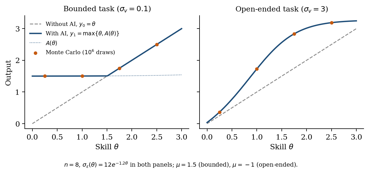
Compression on bounded tasks therefore requires that the AI’s typical output exceed the output of some workers. When it does, those workers are raised to and workers above are unaffected. The left panel of Figure A illustrates the case. The result does not depend on how verification noise varies with skill, because the selection gain is bounded by for every worker.
2.4 The verification premium
Definition 1. For two skill levels , the verification premium is
The premium is the slope of the selection gain between the two workers, measured in units of the slope of unaided output. Since , the premium compares how much more the skilled worker extracts from the AI with how much more that worker produces alone.
Proposition 2. Let . The difference in output between the two workers is larger with AI access than without it, , if and only if and . When both workers use the AI, the difference changes by exactly .
The second condition matters. A premium above one is not sufficient for widening, because if the AI’s mean quality is low enough that neither worker uses it, nothing changes. For example, with , , , , , and , the premium is 1.90 but neither worker adopts and the gap is unchanged. In a sweep of 200,000 random parameter configurations, the statement “the gap widens if and only if ” misclassified 7,597 cases, while the statement in Proposition 2 misclassified none. The proof also shows that whenever only the more skilled worker adopts, the premium necessarily exceeds one.
When is differentiable, the local premium at is , and the gradient of output among workers who use the AI is steeper than one exactly where . Because reliability cannot exceed one, this cannot happen everywhere.
Corollary 1. Suppose is differentiable. The set of skill levels at which has Lebesgue measure less than . If as increases, then along any sequence on which stays bounded.
Amplification is therefore a property of a range of skill, not of a task as a whole. On an open-ended task, AI can widen differences between workers in the middle of the distribution, where verification is improving quickly with skill, while compressing differences at the top, where all workers verify well. The right panel of Figure A shows such a case. This has an empirical implication that we state before turning to data: if amplification occurs, it should be strongest where verification ability is still rising steeply with skill and weaker at the top of the skill distribution.
2.5 Misplaced trust
The analysis so far assumes that workers understand the noise in their own signals. A different and simpler rule is to take the signal at face value. Consider a worker who draws a single candidate () and submits it whenever its signal exceeds the worker’s own output, . Let be the expected gain from AI access under this rule.
Proposition 3. Under Assumption 1 with and the rule “submit the candidate if ”, and writing and ,
As , . As , , which is negative if .
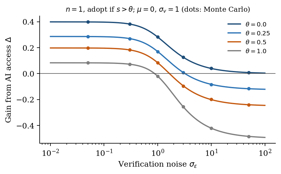
With , and , the gain is 0.197 at , crosses zero at and reaches at , against a limit of . Figure B plots the gain for several skill levels. In every case we computed, the gain falls monotonically in verification noise and crosses zero once, though we have not proved this in general. Proposition 3 rests on a behavioural assumption that differs from the rest of the model. A worker who adopts the candidate only when its posterior mean exceeds can never lose from access, and neither can a worker who makes the ex ante choice behind . Within the model, then, losses of the kind reported by Otis et al. (2026) for low performers, or the errors outside the frontier in Dell’Acqua et al. (2023), can arise only if some users place more trust in what they see than its reliability warrants.
2.6 Comparative statics
To study an automated verifier, suppose that for every candidate the worker also observes , where the are independent draws, independent of everything else, and that the verifier is equally available to all workers and is combined optimally with the worker’s own signal.
Proposition 4. Fix with .
(a) is strictly increasing in , and when .
(b) With an automated verifier, Lemma 1 holds with noise . is strictly increasing in and tends to zero as .
(c) does not depend on .
(d) If , then , and hence , is strictly increasing in .
Part (b) is stronger than the limiting statement. Any improvement in a verifier that all workers share lowers the premium, because reliability is concave in the precision of the information the worker holds and a common addition of precision narrows the difference in reliability between workers. The result requires that skilled and unskilled workers draw the same information from the verifier. If skilled workers make better use of it, the conclusion can fail. Part (c) concerns the premium itself. Whether widening is realised still depends on through the adoption condition in Proposition 2. The condition in part (d) is sufficient but not necessary. In a sweep of 200,000 configurations it never failed when it held, and when it did not hold the gap still rose with in about 72 percent of cases. It can bind: with , and rising from 1 to 1.1, the gap between the two workers falls.
2.7 Skill-dependent prompting and search
So far the mean quality of the AI’s output and the number of candidates are the same for every worker. Skilled users may write better prompts, which raises the mean quality of what they receive, and may draw more candidates before choosing. Let and be nondecreasing, so that , and define the generalised premium
Proposition 5. Let .
(a) The difference in output widens with AI access if and only if and .
(b) Suppose is differentiable with , , and is nondecreasing. The set of skill levels at which is differentiable and has Lebesgue measure less than .
(c) If, on an interval on which is constant and and are differentiable, and , then throughout the interval.
Part (a) shows that the threshold in Proposition 2 carries over unchanged once prompting and search depend on skill. Both channels enter the premium additively, and both raise it. In a sweep of 200,000 configurations in which and rise with skill, part (a) misclassified no case, while the premium of Definition 1, which ignores these channels, misclassified 81,587. Parts (b) and (c) qualify Corollary 1. Amplification remains local as long as better prompting raises mean quality by less than one for one with skill, although the bound on its range grows as . With , and , for example, the premium exceeds one on a skill range of length 4.5 against a bound of 14.2. Once prompting skill raises the quality of AI output at least as fast as it raises unaided output, widening can occur at every skill level. The case for widening on open-ended tasks is therefore stronger when skill also governs how users query the model, and not only how they judge its output.
Remark 1. If the worker can compare the posterior mean of the chosen candidate with after seeing the signals, expected output is , where and is the largest signal. The option value of ex post rejection is itself increasing in reliability, so this extension adds a further source of widening on open-ended tasks. We do not pursue it here.
3Empirical setting and predictions
3.1 Engines as candidate generators and verifiers
Players cannot consult engines during rated games on Lichess, so engines enter chess through preparation and review. A player uses an engine to choose opening lines, to check analysis and to locate mistakes after a game. In the terms of the model, the engine plays two roles. It is a verifier of move quality, because it scores any position it is shown. It is also a generator of candidate lines, because in a given opening it typically offers several continuations whose evaluations are close to equal.
These roles map onto different parts of Proposition 4. For move quality, the engine’s evaluation is the standard against which quality is measured, so the relevant improvement is a better common verifier, which lowers the premium by part (b). We therefore expect the relation between rating and move quality, measured as average centipawn loss, to become flatter. For the choice among engine-equal positions, the engine cannot help by construction, since it evaluates the options as equal. A stronger engine expands the set of lines that survive engine scrutiny, which raises the number of candidates without improving the player’s ability to judge which of them suit a human opponent. By part (a), the premium on this margin rises, and we expect the relation between rating and the quality of this choice to become steeper. Corollary 1 adds that any steepening should be concentrated where verification ability is still rising with rating rather than at the very top.
This mapping is an interpretation, and a demanding one. The model describes a worker who generates candidates with an AI at the moment of production and submits the one that looks best. Engine use is prohibited in rated games on Lichess, so the play we observe is unaided, and engines can affect it only through preparation and review, that is, through what players learn. The model has no learning channel. Our tests therefore ask whether the model’s predictions survive transmission through training: whether a better shared verifier during preparation flattens the rating gradient in what an engine can check, and whether more engine-approved candidates steepen the gradient in what it cannot. A null result is informative about chess and only indirectly informative about the model. The mapping further assumes that the main change between our two periods in how players use engines is the one the model describes, and that the engine-equal positions of the pre period remain informative about practical value in the post period. We return to these assumptions in Section 7.
3.2 Timing
Stockfish 12 was released on 2 September 2020 and was the first release of the engine to use a neural-network evaluation (NNUE) by default (The Stockfish Team 2020b). The NNUE evaluation had been merged into the public development code on 6 August 2020 (The Stockfish Team 2020a). Lichess, the source of our data, switched its server-side analysis to Stockfish 12 with NNUE on 27 November 2020, continued to accept analysis from volunteer machines running the older engine until early January 2021, and reported that all standard games were analysed with NNUE by mid-January 2021 (lichess-org 2020, n.d.; Lichess 2021). The months between March 2020 and August 2021 also include the start of the pandemic and a large inflow of new players. We exclude March 2020 through August 2021 and compare January 2018 to February 2020 with September 2021 to October 2023, two windows of 26 months each.
4Data and measures
4.1 Games and sample
We use the monthly files of standard rated games published by Lichess (Lichess, n.d.-b). We stream each file and keep rapid and classical games according to Lichess’s own speed categories, which classify games by an estimated duration equal to the initial time plus 40 times the increment (Lichess, n.d.-a). Files from early 2018 label the rapid category “Standard”; the label covers the same range of estimated durations and we code it as rapid. For each game we record the players, their pre-game ratings, the result, the date, the time control, the first 30 half-moves and, where the game has been analysed by Lichess, the engine evaluation after every move.
Accounts are split by a hash of the username. Half of all accounts are reserved for estimating the properties of opening positions and are never used in the regressions. The estimation sample is drawn from the other half. A player enters the balanced panel if they have at least ten rapid or classical games in each period. For storage and computation, the estimation sample consists of a random five percent of all accounts, selected by the same hash and lying entirely in the non-reserved half. The balanced panel contains players and player-game observations in rapid and classical games. Of these, observations come from analysed games with at least ten scored moves and carry a move-quality measure, and carry a practical-choice score. Lichess’s files for March and April 2018 both contain the 5,502 games played on 31 March 2018; we keep one copy of each, and no other game appears in more than one file. Panel players were rated 1,544 on average in the early window and 1,734 in the later one, so ratings rise within player over the sample; we return to this drift below.
4.2 Move quality
We measure move quality by average centipawn loss (ACPL), computed from the evaluations that Lichess attaches to analysed games. For each move we take the drop in evaluation from the mover’s point of view, set to zero when the evaluation improves, after clamping evaluations at centipawns and treating forced mates as . A player’s ACPL in a game is the mean of these losses over their moves, excluding White’s first move. We require at least ten scored moves.
Two features of these evaluations shape our design. First, only games that someone has asked Lichess to analyse carry evaluations, and the share of analysed games rises with rating. In January 2018 it was 13 percent for games between players rated below 1400 and 49 percent for games between players rated 2200 or above. Second, the engine behind the evaluations changed between our periods, from the classical Stockfish evaluation to NNUE, and it changed again within the post period. Lichess’s analysis client adopted Stockfish 15.1 on 4 December 2022 and Stockfish 16 in July 2023 (lichess-org, n.d.), and Stockfish 15.1 introduced a convention under which an evaluation of +1 corresponds to a 50 percent chance of winning against an equal opponent, which the developers describe as scaling evaluations down somewhat (The Stockfish developers 2022). A uniform rescaling of evaluations multiplies ACPL by a constant, which would change the slope of ACPL on rating in levels but is absorbed by month fixed effects in logs. Our primary outcome is therefore the logarithm of ACPL. To address both the change in engine and selection into analysis, we also re-evaluate a stratified random sample of 8,000 panel games, drawn from all games and not only analysed ones, with a single fixed engine (Stockfish 17.1 at 200,000 nodes per position). This sample is small next to the main one. Before seeing its results we predicted that its standard error would be roughly 15 times larger than that of the main estimate; it turned out to be about 4 times larger without player fixed effects and about 6 times larger with them (Appendix B).
4.3 Engine-equal positions and outcome skew
Our second outcome follows Park (2026), who shows that among opening positions an engine rates as equal, some favour White and others Black in actual play, and that these differences replicate across disjoint groups of players. We construct the measure from pre-period games between accounts in the reserved half. We identify opening positions reached within the first 30 half-moves at least 200 times, merging move orders that transpose to the same position, and evaluate each with a fixed build of Stockfish 17.1 at depths 20, 25 and 30. A position is engine-equal if its evaluation lies within 10 centipawns of zero at all three depths.
We then fit an expected-score model in the reserved sample, following Park (2026). White’s score, with draws counted as one half, is modelled by a fractional logit in a natural cubic spline of the rating difference, the mean rating of the two players, their interaction, speed indicators and speed-specific slopes on the rating difference. The skew of a position is the mean residual of White’s score across games that reach it. To check that skews measure something stable, we split the reserved accounts again into two groups, estimate skews separately in each, and regress one set on the other after removing opening-family means, as Park (2026) does. The reserved sample contains pre-period games between reserved accounts. We evaluate all 64,323 positions reached at least 200 times at depth 20, and the whose depth-20 evaluation lies within 25 centipawns of zero also at depths 25 and 30. This leaves engine-equal positions under our rule and under the looser rule of Park (2026), which requires the three evaluations to agree within 50 centipawns and the depth-30 evaluation to lie within 10 centipawns of zero. Across positions in opening families with at least 200 games in each half, the split-half slope is (95 percent confidence interval to ), against (0.646 to 0.736) in Park (2026) for October 2025 and in his rapid games alone. The median absolute skew is , or about three percentage points of expected score. Our larger sample, 26 months against one, is a likely reason for the higher reliability, though we have not tested this. On the half-B games of October 2025, the month Park studies, our skews for the same positions replicate with a slope of (95 percent confidence interval to ) across 365 positions with enough games, between his rapid and overall estimates; his sample also includes blitz, and his engine-equal positions are his own.
The practical-choice score of a player in a game is the skew of the first engine-equal position that arises immediately after one of the player’s own moves, signed so that positive values favour the player. It is missing when no such position arises. The score uses only pre-period skews estimated on other players, so it does not mechanically reflect the outcome of the game in which it is measured.
5Empirical strategy
For player in game played in month , we estimate
where is the player’s pre-game rating in hundreds of points centred at 1500, indicates the later window, and are player and month fixed effects, and contains the opponent’s rating, the player’s colour and time-control fixed effects. Standard errors are clustered by player. The coefficient is the within-player gradient of the outcome in rating before the engine shock and is its change afterwards. Our predictions are and for log ACPL, and and for the practical-choice score. We wrote these predictions, the full specification and the robustness checks into an analysis plan before computing any outcome on the estimation sample, and committed it to a version-controlled repository (commit 7bd6c20, 13 November 2026, 23:31 UTC). The repository is private, so this timestamp cannot be verified externally, and the plan should not be read as a public pre-registration (Appendix B).
The design has no untreated group. Every player could use the new engine, so captures any change in the rating gradient between the two windows, of which the change in engines is one candidate cause. We probe this with placebo break dates inside the pre period, an event-study version that traces the gradient quarter by quarter, and splits by rating band.
6Results
6.1 Move quality
Table 1 reports the main estimates. In the first column the outcome is log ACPL. Before the engine shock, a gain of one hundred rating points within a player is associated with a percent lower average centipawn loss (). In the later window this gradient is smaller in absolute value by (standard error , 95 percent confidence interval to ), a flattening of percent. Taken alone, the estimate has the sign predicted by H1 and is precisely estimated.
| Log ACPL | Practical-choice score (pp) | |
|---|---|---|
| Rating () | ||
| Rating Post () | ||
| Holm-adjusted for | ||
| Observations | 1,752,929 | 2,020,879 |
| Players | 12,407 | 12,391 |
| Player, month and time-control FE | Yes | Yes |
Notes: Each column reports one regression of the outcome on the player’s rating (hundreds of points, centred at 1500), its interaction with an indicator for September 2021 to October 2023, the opponent’s rating and the player’s colour, with player, month and time-control fixed effects. Standard errors clustered by player in parentheses. , , : , , . The practical-choice score is in percentage points of expected score. The predictions are for log ACPL and for the practical-choice score.
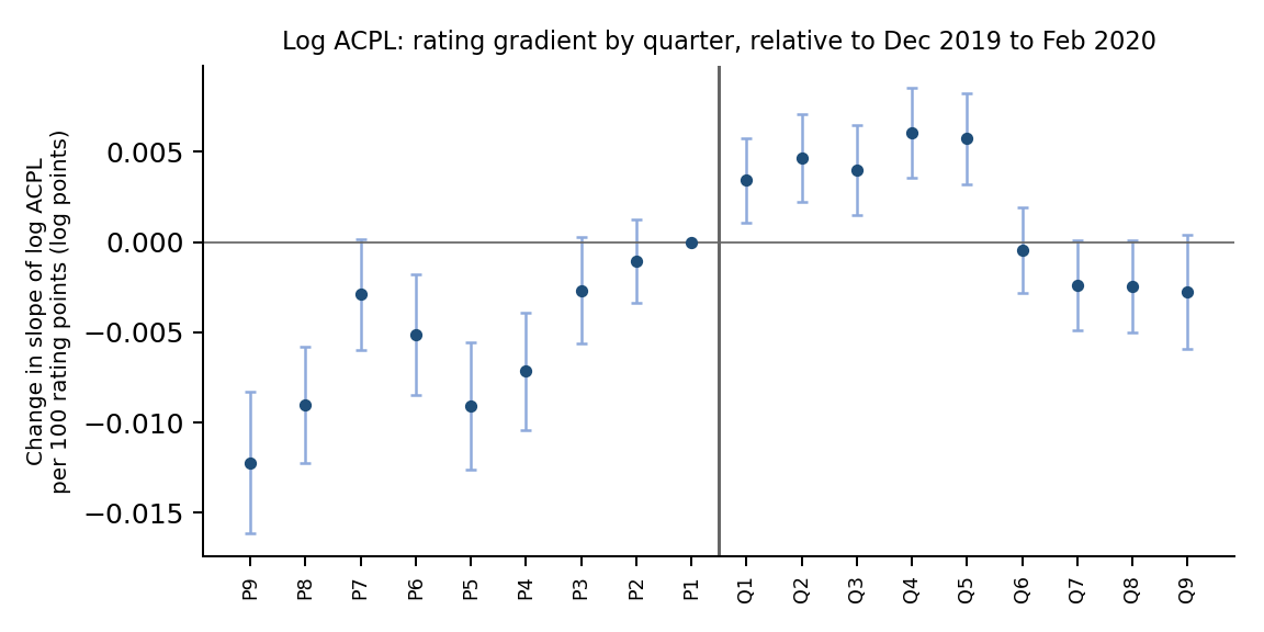
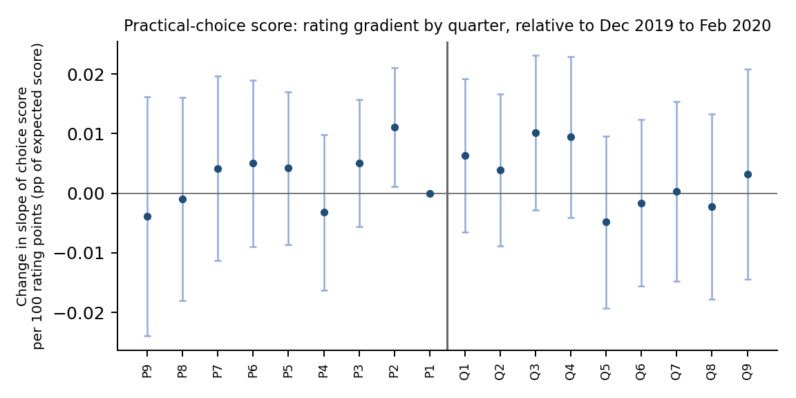
The pre-specified placebo tests do not support reading this estimate as a response to the engine. Using only pre-period data and a fake break in July 2018, the same specification gives a change of (standard error ); with a fake break in August 2019 it gives (). Both are at least as large as the estimate at the real break. Figures C and D show why. The top panel replaces the single post indicator with interactions between rating and quarter of the sample, relative to December 2019 to February 2020. The coefficients rise steadily through the pre period, from about in early 2018 to zero in the reference quarter, which means that the gradient was flattening well before Stockfish 12. The first five post-period quarters lie above the reference level by to . A linear continuation of the pre-period trend, which rises by about per year, would place them higher still, so these quarters show no excess flattening relative to that trend. The coefficients then fall below zero from December 2022 onward, which is when Lichess’s analysis client moved to Stockfish 15.1 with its new evaluation scale. Since all evaluations in our data come from the engine Lichess was running at the time, this second change is a plausible source of the drop, although we cannot rule out other causes.
Two further pre-specified checks point the same way. Without player fixed effects the change in the gradient is (), so the cross-sectional relation between rating and move quality did not flatten at all, and the within-player estimate is not mirrored across players. Within rating bands defined by the pre-period mean rating, the change is close to zero below 1400 and negative between 1400 and 2200 ( and ), the opposite of the prediction. The robustness checks that address the measurement of move quality leave the pooled estimate similar: rating as a within-month percentile, cell fixed effects for rating band by month to absorb changes in who requests analysis, and ACPL in levels all give positive changes, between 21 and 41 percent of the pre-period gradient (Appendix B). These checks do not address the pre-trend.
Following our analysis plan, we report H1 as not supported. The pre-specified estimate has the predicted sign, but the placebo tests we specified to validate it fail, and the event study shows that the change predates the engine. After seeing these results we also estimated three exploratory variants, which were not in the plan (Table 5). Ending the later window in November 2022 raises the estimate to , and adding a linear trend in the rating gradient over the full sample gives , since the late decline flattens the fitted trend. Combining the two, so that the trend is estimated without the period after the second engine change, gives (). The sign of the estimated break thus depends on how the pre-existing trend is modelled, which is a further reason not to interpret it.
6.2 Practical choice
The second column of Table 1 reports the results for the practical-choice score, in percentage points of expected score. Higher-rated players reach engine-equal positions that score better in practice: before the shock, one hundred rating points within a player raise the skew of the first engine-equal position after the player’s own move by percentage points. This is small next to the median absolute skew of about three percentage points, so most of the variation in the positions players reach is unrelated to their rating. The change in the gradient after the shock is (standard error ), with a 95 percent confidence interval from to . Relative to the pre-period gradient, the interval runs from to , so we can exclude a steepening or flattening of more than about 13 percent. The bottom panel of Figures C and D show a flat profile before and after the break, the placebo breaks give estimates of zero, and the estimate stays close to zero when skews are estimated within rating bands, shrunk toward zero, or computed on the looser set of engine-equal positions used by Park (2026). H2 is not supported. The secondary prediction H3, that any steepening would be concentrated in the middle of the rating distribution, is also not supported: the band estimates are , , and from the lowest band to the highest, none of them distinguishable from zero.
The coverage of the choice score is stable. Between 12 and 17 percent of observations in each rating band and period carry a score (Table 2), and the shares barely move between windows. The share of games with engine evaluations rose in every band, from 12.8 to 16.2 percent overall.
| Has evaluations | Has choice score | |||
|---|---|---|---|---|
| 2-3(lr)4-5 Rating at game | Pre | Post | Pre | Post |
| 1400 | 0.118 | 0.143 | 0.158 | 0.171 |
| 1400-1800 | 0.124 | 0.144 | 0.171 | 0.172 |
| 1800-2200 | 0.152 | 0.171 | 0.150 | 0.157 |
| 2200 | 0.293 | 0.344 | 0.125 | 0.122 |
Notes: Shares of player-game observations in the balanced panel.
6.3 Exploratory evidence added after review
The analyses in this subsection were specified after the main results had been seen and after an external review of the first draft. They address questions that the pre-specified design leaves open, and we report them as exploratory (Table 3).
The first asks whether the engine shock changed how these players open games at all, since a null result means little if the treatment did not reach them. We measure, for every panel game, how long the game stays within lines that were frequent in the pre period, whether it has left them by the twelfth half-move, and whether it reaches any engine-equal position. On average, games stay in frequent lines for 7.8 half-moves before the break and 7.9 after; 91.3 and 90.6 percent leave them by the twelfth half-move; and 24.9 and 24.7 percent reach an engine-equal position. Within rating bands the only visible change is in the 1800–2200 band, where the share leaving frequent lines by the twelfth half-move rises from 86.7 to 89.0 percent and the entropy of the first ten half-moves, computed on equal subsamples of 20,000 games, rises from 9.43 to 9.57. Entropy rises slightly above 2200 (9.01 to 9.10) and is flat below 1800. Because these measures are defined relative to lines that were frequent before 2020, they can register a move away from old lines but not the content of new ones. With that caveat, we find little evidence that opening play changed for most of the players in our panel.
The second analysis measures the choice itself. The practical-choice score records where a player ends up, which also depends on the opponent’s moves. A more direct measure looks at positions from which at least two moves lead to engine-equal positions, and asks which of them the player picks. There are 553 such positions in the frequent pre-period lines, each with 2.3 engine-equal continuations on average and a median difference of 2.5 percentage points of expected score between the best and the worst of them. Panel players face these positions 8.7 million times and choose one of the engine-equal moves in 15.5 percent of cases. When they do, they choose the highest-skew move 43.9 percent of the time, against 42.9 percent under random choice among the engine-equal moves, and the chosen move’s skew exceeds the average of the options by 0.35 percentage points. Players as a group therefore lean slightly toward the better option, and the lean rises only negligibly with rating. Within players, a hundred rating points change the probability of choosing the best move, net of chance, by (standard error ), which is indistinguishable from zero, and raise the demeaned skew of the chosen move by percentage points (). The second gradient is clearly different from zero but small: it amounts to about half a percent of the median spread between the options per hundred rating points. Neither gradient changed after the shock. In the terms of the model, the reliability with which players judge engine-equal options rises with skill, but only slightly.
The third analysis probes the pre-trend in the move-quality gradient. If it comes from players who are early in their careers and improving quickly, it should be concentrated among newer accounts. Creation dates from the public Lichess user API could not be retrieved in bulk because of rate limits, so we proxy newness by first appearance in our rapid and classical data: players with no such game in January to June 2018 count as new. Among the 7,929 new players, the change in the gradient is and the placebo break in August 2019 gives a larger . Among the 4,478 established players, the change is () and the placebo gives (). The pre-trend is thus concentrated among newer players, as the career explanation predicts. Among established players the estimate at the real break exceeds the placebo, but the two are of similar size, the placebo covers a shorter window, and comparing them was not part of our design, so we do not read this as evidence for H1. Restricting the sample to players whose mean rating changed by less than 100 points between windows removes most of the within-player variation in rating (, not distinguishable from zero), and the placebo again exceeds the estimate at the real break.
A fourth analysis, prompted by a second review, asks whether curvature explains the pattern of the pre-specified estimates. The pooled change in the move-quality gradient is positive, while every band-specific change is zero or negative. A linear gradient fitted to a relation that is curved in rating would flatten as players move up the rating scale, with no engine involved. The relation is indeed curved. In a piecewise-linear specification with knots at 1400, 1800 and 2200 that lets every segment change after the break, the pre-period slope of log ACPL is per hundred points below 1400, about between 1400 and 1800, and about between 1800 and 2200; Panel C of Table 3 reports the specification with a single common change, in which the slope below 1400 is . Allowing for this curvature cuts the pooled change at the real break from to (), so curvature accounts for more than half of the pre-specified estimate and for its disagreement with the band splits. It does not account for the pre-trend. With the same spline, the placebo breaks in July 2018 and August 2019 give and , close to their values without it. The estimate at the real break is now about a third of the estimates at the two placebo dates, which is the clearest evidence in the paper against attributing the flattening to the engine (Panel C of Table 3). When every segment of the spline may change after the break, the change is concentrated below 1400 (, standard error ), falls to about between 1400 and 1800 and is about zero between 1800 and 2200, which fits the finding that the drift comes from newer, lower-rated players.
| (s.e.) | (s.e.) | Obs. | |||
|---|---|---|---|---|---|
| A. Choice at branch points (parent-position fixed effects) | |||||
| Demeaned skew of chosen move (pp) | 1,347,129 | ||||
| Chose the highest-skew move, minus chance | 1,347,129 | ||||
| Chose an engine-equal move (quarter of players) | 2,259,708 | ||||
| B. Log ACPL by newness to rated slow play | |||||
| First seen July 2018 or later | 941,102 | ||||
| placebo break, August 2019 | 318,048 | ||||
| Active January–June 2018 | 811,827 | ||||
| placebo break, August 2019 | 191,212 | ||||
| Mean rating change below 100 points | 367,197 | ||||
| placebo break, August 2019 | 105,931 | ||||
| C. Log ACPL with a piecewise-linear rating spline (knots at 1400, 1800, 2200) | |||||
| Real break, common change in slope | 1,752,929 | ||||
| placebo break, July 2018 | 300,928 | ||||
| placebo break, August 2019 | 509,260 | ||||
Notes: Not part of the analysis plan; specified after the main results and an external review were seen. Each row is one regression with the controls and fixed effects of Table 1 (Panel A adds fixed effects for the parent position). is the coefficient on rating and on rating post (or placebo post). Panel A uses 553 positions from which at least two moves lead to engine-equal positions; the first two rows are defined where the player chose one of them. Panel B splits players by first appearance in our rapid and classical data, a left-censored proxy for account age. In Panel C, is the slope below 1400 and the spline terms are included but not shown. Standard errors clustered by player. , , : , , .
7Discussion
7.1 Why the predictions may fail in this setting
The null results admit several readings. The exploratory evidence helps to separate them, though not conclusively.
The first reading is that the shock was small on the margins we measure. Stockfish 11 already played far above any human level, so for the moves of club players its evaluations and those of Stockfish 12 should agree on almost every blunder and almost every good move. The improvement in the external verifier may have been large in absolute strength but small in the range of quality that matters for the players in our panel, in which case Proposition 4 predicts little change in the premium. Opening preparation with strong engines was also widespread before 2020. The first-stage evidence is consistent with this reading: how long games stay in established lines, how often they leave them early and how often they reach engine-equal positions barely changed between windows, with a modest increase in novelty only between 1800 and 2200.
The second reading concerns the practical-choice margin itself, and here the first draft of this paper drew the wrong conclusion. The median absolute skew of the positions players reach is about three percentage points of expected score, and the split-half reliability of 0.72 implies that most of this variation reflects real differences between positions. The dispersion of candidate quality, in the model, is therefore not small, and the margin is not a bounded task in the sense of Proposition 1. What is small is the gradient of choice quality in rating. The branch-point analysis shows directly that, given a choice between engine-equal moves, players of all ratings pick the one that does better in practice only slightly more often than chance, and higher-rated players do better only to a negligible degree. In the model’s notation, is small, though measurably positive, on this margin: players at every rating have little ability to tell which engine-equal option suits a human. Since the premium is proportional to , it stays small however many candidates the engine supplies, and the model then predicts little or no widening. The choice among engine-equal openings is thus open-ended but unverifiable for human players, which is a more informative finding than a bounded task would be. It also means that this margin could not have delivered the test we designed, since an increase in raises the premium only where verification ability rises with skill. This reading was formed after seeing the results, and we offer it as such.
The third reading concerns identification. The design has no group that was denied the new engine, so captures every change in the rating gradient between the two windows. The pre-trend in the move-quality gradient shows that such changes occur without any engine shock. The exploratory analyses suggest where it comes from. The pre-trend is concentrated among players who were new to rated slow play in 2018, whose ratings rise quickly and whose relation between rating and move quality may change as they gain experience. Log ACPL is also convex in rating, so a linear gradient flattens as players move up; allowing for this curvature removes more than half of the pre-specified estimate but leaves the placebo changes nearly intact. Panel players as a whole gain about 190 rating points between windows. The selection of games into analysis also shifts, since the share of analysed games rose in every rating band. Our pre-specified controls for these channels, rating percentiles and band-by-month fixed effects, change little, but they cannot rule out every form of drift.
The fourth reading concerns measurement. Every evaluation in the Lichess files was produced by whichever engine Lichess was running when the game was analysed, so move quality in the early window is measured with classical Stockfish, in the later window with NNUE, and from December 2022 with the rescaled evaluations of Stockfish 15.1. Logs absorb a uniform rescaling but not a change in how the engine ranks small errors, and the timing of the decline in the event study suggests that the 2022 change mattered. The fixed-engine re-analysis removes this channel for a random sample of 8,000 games. Its like-for-like estimate, with player fixed effects, is with a standard error of , consistent with the main estimate but also with zero, and its version without player fixed effects disagrees with the corresponding main estimate by almost three standard errors (Appendix B). The check therefore cannot rule the engine channel in or out, and it cannot speak to the pre-trend.
7.2 What the results imply for the model
The model is a statement about selection among AI outputs at the moment of production, and online chess tests it only through the indirect channel of preparation. Within that limit, the evidence is negative in a specific sense. It does not contradict the model: on the margin an engine cannot verify, the premium appears to be near zero because human verification does not improve with skill, and in that case the model predicts no widening. Nor does it support the model, because neither prediction was confirmed and the setting lacks a comparison group.
A sharper test would use a setting in which people choose among engine or AI outputs while producing, and in which the shared verifier changes at a known date. Correspondence chess under the International Correspondence Chess Federation comes close. Engine use is permitted, players generate candidate moves with engines and choose among them, and the arrival of NNUE improved the verifier available to everyone at once. Proposition 4 predicts that a better common verifier lowers the premium and so compresses differences between players who use it, a prediction we have not examined in those data. ICCF game records are not distributed as a single public database; individual championship files and commercial compilations exist, and we leave this test to future work. Field experiments with randomised access to generative AI offer the other route, and the model’s main empirical implication, that the sign of the effect on inequality depends on the verification premium, is best tested there by measuring the dispersion of candidate quality and verification skill directly.
8Conclusion
We have proposed a model in which generative AI raises output through selection among candidates, and the gain from selection depends on how well the user can verify them. The model separates the mean quality of the tool from a selection gain that depends on skill, gives an exact condition for AI to widen differences between workers, and shows that such widening can occur only over a bounded range of skill unless better prompting raises the quality of AI output at least one for one with skill. This locality result offers one way to reconcile field experiments that find compression with those that find widening.
Our attempt to test the model’s predictions in online chess around the release of Stockfish 12 did not find support for them. The rating gradient in move quality flattened between 2018 and 2023, but it was flattening before the engine arrived, mainly among newer players, and the placebo tests we specified in advance reproduce the change. Allowing for the curvature of move quality in rating makes the point sharper: the change at the real break shrinks to , about a third of the changes at the placebo dates. The gradient in the choice among engine-equal openings did not change, and exploratory evidence indicates that players at every rating have little ability to tell which engine-equal option suits a human and that this ability barely rises with rating, which in the model leaves little premium for more candidates to amplify. Because engines are not used during rated games, these tests reach the model only through preparation. We read the results as a careful negative application, informative about how engine improvements did and did not reach club play, and we regard engine-assisted correspondence chess and experiments that measure candidate dispersion and verification skill directly as the more promising routes to a test of the theory itself.
Appendix A. Proofs
Proof of Lemma 1. Conditional on the vector of signals, depends only on , because is independent of for . Since is jointly normal with and ,
which is nondecreasing in , so the candidate with the largest signal maximises the conditional expectation of the submitted value. Write for its index. By the law of iterated expectations, . The signals are independent draws, so . Hence . When the same argument applies with . ◻
Proof of Proposition 1. For every , , so . Since is 1-Lipschitz, for all , which tends to zero. For the gap, equals if , equals if , and equals if . ◻
Proof of Proposition 2. Write , and , and note . Consider the four adoption cases. If and , the gap is . If and , the gap is , which exceeds if and only if , and the change is . If and , the gap is . If and , the gap is ; in this case , so . Hence the gap exceeds in exactly two cases, both of which have and . Conversely, suppose and . If we are in the second case and the gap widens; otherwise we are in the fourth case and the gap widens. If instead and , then , so neither worker adopts and the gap is unchanged. ◻
Proof of Corollary 1. Let . Since is nondecreasing and differentiable, and . Then when , which gives the bound; because . For the second statement, , which tends to zero when and is bounded. ◻
Proof of Proposition 3. Output is if and otherwise, so . Here and . Therefore
using . As , and , and the expression converges to , which is strictly positive because has full support. As , , and , so . ◻
Proof of Proposition 4. (a) is proportional to with a positive factor. The sequence is strictly increasing because with strict inequality on a set of positive probability, and .
(b) The pair is equivalent, for inference about , to the precision-weighted average with , independent across candidates, so Lemma 1 applies with . Write reliability as a function of precision , . Direct differentiation gives and . With and , , which is strictly decreasing in because is strictly decreasing, and tends to zero as because . Since is decreasing in , is strictly increasing in and tends to zero as . (If , and the same argument applies with .)
(c) does not appear in .
(d) with and , so . Then and , so is strictly decreasing in for . If , then and the derivative of the gap with respect to is positive. ◻
Proof of Proposition 5. (a) The proof of Proposition 2 uses only through the four adoption cases and the identity . Both hold with in place of for any function , so the argument applies verbatim.
(b) Let , which is nondecreasing, takes values in , and is differentiable wherever is. Let be the set of points at which is differentiable and . On , . For a nondecreasing function the integral of its derivative over any measurable set is at most its total increase, so when .
(c) On the interval, with for , so . ◻
Appendix B. Robustness checks specified in the analysis plan
We wrote the analysis plan in results/analysis_plan.md before computing any outcome on the estimation sample, and recorded every later change in its changelog. Before the full run, we executed the estimation code once on two months of data (January 2018 and September 2021) to find programming errors; those estimates were not used, and no hypothesis, outcome or specification changed afterwards. Implementation details that the plan left open are as follows. The estimation sample is the five percent of accounts with the lowest hash values, a random subset of the non-reserved half. The expected-score model is fitted on a random sample of three million reserved games, with spline knots placed at quantiles of a random subsample of 200,000 of them. Practical-choice scores use positions reached at half-moves 2 to 30. The secondary hypothesis H3 refers to “middle bands”; we compare the 1400–1800 and 1800–2200 bands with the band at 2200 and above.
Table 4 reports all pre-specified checks except the event study, which appears in Figures C and D. For move quality, the placebo breaks reproduce the main estimate, the cross-sectional specification without player fixed effects shows no change, and the band splits show changes of the opposite sign in the middle of the rating distribution. Tournament games, where the decision to request analysis may be less selective, give a smaller and insignificant change of () on a sample about one sixteenth the size of the main one. For practical choice, every variant gives an estimate close to zero.
| Move quality | Practical choice | |||
|---|---|---|---|---|
| 2-3(lr)4-5 Specification | (s.e.) | (s.e.) | ||
| Placebo break, July 2018 (2018-01 to 2019-01) | ||||
| Placebo break, August 2019 (2019-01 to 2020-02) | ||||
| Players rated below 1400 (pre-period mean) | ||||
| Players rated 1400–1800 | ||||
| Players rated 1800–2200 | ||||
| Players rated 2200 or above | ||||
| Skews estimated within rating bands | ||||
| No player fixed effects | ||||
| Rating band month fixed effects | ||||
| Tournament games only | ||||
| ACPL in levels | ||||
| Fixed-engine ACPL, no player FE (log) | ||||
| Fixed-engine ACPL, no player FE (levels) | ||||
| Fixed-engine ACPL, player FE (log) | ||||
| Fixed-engine ACPL, player FE (levels) | ||||
| Rating as within-month percentile (deciles) | ||||
| Shrunken skews | ||||
| Engine-equal set defined as in Park (2026) | ||||
Notes: Each entry is the coefficient on rating post (or on rating placebo post) from a separate regression with the controls and fixed effects of Table 1 unless stated otherwise. Move quality is log ACPL except where noted. Standard errors clustered by player. Rating bands use the player’s mean pre-period rating.
The fixed-engine re-analysis re-evaluates 8,000 randomly sampled panel games, drawn from all games and stratified by period and rating band, with Stockfish 17.1 at 200,000 nodes per position, and recomputes ACPL with the same rule as in the main analysis. The analysis plan specified two versions, one with month and time-control fixed effects and one adding player fixed effects where the sample allows, without naming either as primary. The version with player fixed effects is the like-for-like comparison with the main estimate. Its change in the gradient of log fixed-engine ACPL is (standard error , 95 percent confidence interval to ), an interval that contains both zero and the main estimate of . Most sampled players contribute only one or two games, so this version rests on few within-player comparisons. Without player fixed effects the change is (), but this regression measures something different: its pre-period gradient is , about four times the within-player gradient of the main specification. Its natural comparison is the main panel without player fixed effects, where the change is (). The two differ by about 2.8 standard errors. Different samples could explain the gap, since the re-analysis includes games nobody asked Lichess to analyse and weights the four rating bands equally, but so could a difference between how Lichess’s changing engines and the fixed engine measure quality, which would mean that the change of engine does affect the main estimates. In levels without player fixed effects the change is (). Before the re-analysis ran, we predicted that its standard error would be about 15 times that of the main estimate. It is about 4 times larger without player fixed effects and about 6 times larger with them, so the prediction was too pessimistic. Overall, the fixed-engine check is consistent with the main estimate but cannot rule the engine channel in or out. It also covers the two windows only, so it cannot address the pre-trend, and it does not change our reading of H1.
Table 5 reports the three exploratory variants discussed in Section 6. They were chosen after the pre-specified results were seen, to probe the timing of the decline in the move-quality event study and the pre-trend, and we do not use them to test any hypothesis.
| Log ACPL | Practical choice (pp) | |||
|---|---|---|---|---|
| 2-3(lr)4-5 Specification | (s.e.) | (s.e.) | ||
| Later window ends November 2022 | ||||
| Rating linear trend, full sample | ||||
| Both of the above | ||||
Notes: Chosen after the pre-specified results were seen. Each entry is the coefficient on rating post from the specification of Table 1, with the change indicated. The linear trend is rating interacted with years since January 2018. Standard errors clustered by player. , , : , , .