What Does a Change Detector Find Where Nothing Changed?

Abstract

A change detector is easy to make look good, because the quantity that would expose it is the one nobody measures. Every parameter that raises the count of changes found also raises the count of changes imagined, there is no labelled ground truth for an arbitrary square kilometre of the earth, and the field's standard metrics are structurally unable to score the case where the correct answer is nothing. This note measures the false-alarm rate from the other end: run the pipeline over ground whose invariance a different community has already certified, and report what comes back. The registry exists, is maintained by CEOS for radiometric calibration, and has been independently shown stable to within 0.215% in top-of-atmosphere reflectance per year, so the null is defended before the experiment starts. The practice is standard in observational astronomy, where it is called a null test, and absent from Earth observation, where the official change-map validation protocol does not contain the word invariant. I argue the absence is structural rather than accidental: on an empty ground truth, F1 and intersection-over-union are undefined for a perfect result and identically zero for every imperfect one, so they cannot separate one false positive from five hundred thousand. Measuring what automatic thresholds return on signal-free input, common selectors report between 2.83% and 50.12% of an empty scene as changed, and Otsu's rate does not decay but falls 26.97 percentage points across a single 0.25σ step in signal contrast, so behaviour on scenes containing change predicts nothing about behaviour on scenes without it. On real Sentinel-2 imagery over the six CEOS-endorsed sites, a purely data-driven threshold reports a median of 21.41% of certified-invariant desert as changed, against 0.04% with an absolute floor. Running the protocol against a working pipeline surfaced seven defects, five of which are invisible in the outputs.

1You cannot label the earth

Ask a change-detection system what happened between two passes over a square kilometre of anywhere, and you will get an answer. Ask how often that answer is wrong and the question becomes strangely hard.

The obvious route is the one the field takes: annotate pairs of images by hand, count what the system got right and wrong against the annotation, and report precision and recall. This works, it is what the benchmarks are built from, and it has an obvious ceiling. Annotation is expensive, so benchmarks are small and geographically narrow. They age. And a system tuned until it scores well on an annotated benchmark has been tuned to agree with a particular set of annotators about a particular few cities, which is not the same as being right about the earth.

There is a second problem, less obvious and worse. Every knob that makes a detector find more real change also makes it find more imaginary change. The two move together, and only one of them is measured by a benchmark consisting of scenes where something happened. A system that reports a great deal of change is, from the outside, indistinguishable from a system that works.

What follows is a way of measuring the second quantity that costs nothing, scales without limit, and requires no one to annotate anything. It is not a new idea. It is an old idea from a different field, and an existing asset from an adjacent one, put together.

2The null test

In observational astronomy and cosmology, a measurement is not trusted until it has survived a null test. The construction is always the same: arrange the data so the real signal cancels, then look at what is left. Split the observations in half and difference them, and any genuine sky signal disappears, so the residual power is systematics and nothing else. Experiments like Planck and the South Pole Telescope run suites of these, and passing them is a precondition for claiming a detection rather than an optional extra. A recent stellar-stream algorithm states the criterion plainly: the method is run on a field with the stream removed, and a perfect method should yield zero detections in the null test.

The Earth-observation equivalent is available and unused. Since the late 1980s, satellite radiometry has relied on the fact that some ground does not change. Schott, Salvaggio and Volchok introduced pseudoinvariant features for exactly this reason, and Cosnefroy, Leroy and Briottet selected twenty Saharan and Arabian sites of 100 by 100 kilometres with spatial uniformity better than 3%. Six are now endorsed by the Committee on Earth Observation Satellites as standard reference targets: Libya-1, Libya-4, Algeria-3, Algeria-5, Mauritania-1 and Mauritania-2. They are used continuously to track sensor drift, and the catalogue is maintained by the USGS.

The crucial property is that their invariance has been argued by somebody else, adversarially, in public. Khadka, Teixeira Pinto and Leigh ran change-point detection on the sites themselves, specifically to test whether calling them invariant is safe, and found a maximum trend of 0.215% in top-of-atmosphere reflectance per year. Tuli and colleagues caution in the same literature that stability cannot be assumed and should be regularly monitored.

That is the difference between this and pointing a detector at somewhere quiet. An ad-hoc choice of an empty-looking place is an assumption. A CEOS-endorsed site is a published, defended, periodically re-tested claim that a third party staked their instrument calibration on. The null is established before the experiment begins, and by people with no interest in this paper's conclusion.

The protocol. Select null sites from the certified registry rather than by inspection. Acquire pairs at several temporal separations. Run the complete pipeline unmodified, with production settings. Report the detected area fraction per site as a distribution. And report an expectation rather than assuming zero, following the cosmology practice, because a null site is radiometrically stable rather than physically frozen.

3Why the field could not have done this

The absence is easy to document. The CEOS Working Group on Calibration and Validation publishes the good-practices protocol for assessing the accuracy of land-cover and change maps. It is the doctrine, from the same organisation that curates the invariant sites. A full-text search of the 2025 edition returns zero occurrences of invariant, zero of pseudo-invariant, zero of stable site, zero of control site, and zero of false alarm. The sanctioned method is probability sampling with human reference interpretation. A 2025 review of operational change detection puts it from the other direction, in a section titled The unstudied no-change detection: no established method currently exists.

It would be easy to read that as an oversight. It is not. The field's instruments cannot express the measurement.

Take a scene pair where nothing changed. The ground truth mask is empty, so true positives and false negatives are both zero by construction. Now compute the standard metrics as a function of how badly the detector failed, on a scene of a million pixels:

false positives	precision	recall	F1	IoU	overall accuracy
0	0/0	0/0	0/0	0/0	1.0000
1	0.000	0/0	0.000	0.000	1.0000
100	0.000	0/0	0.000	0.000	0.9999
10,000	0.000	0/0	0.000	0.000	0.9900
100,000	0.000	0/0	0.000	0.000	0.9000
500,000	0.000	0/0	0.000	0.000	0.5000

Recall is zero over zero always, because its denominator is empty. F1 and intersection-over-union are undefined for a perfect null result and exactly zero for every imperfect one. They have no discriminative power at all in this regime: a detector that hallucinates a single pixel and one that hallucinates half the scene receive the same score. The only metric that moves is overall accuracy, which is precisely the number the change-detection literature has taught itself to distrust, because on ordinary scenes it is dominated by the unchanged class and flatters everything.

This is, I think, the whole explanation. A research community cannot report a quantity its metrics return as zero over zero, cannot rank methods by a number that is constant, and will not build benchmarks for a case it cannot score. The gap is not a blind spot in the field's attention. It is a hole in the field's ruler.

The corollary is that a null test needs a different reported quantity, and the natural one is the fraction of the scene reported as changed. It is defined everywhere, zero when the detector is right, monotonic as the detector gets worse, and needs no labels. Ren and colleagues brushed against this in a single subsection, noting of a no-change pair that no PR or ROC curves can be plotted and that only overall accuracy could be calculated, but treated it as an inconvenience rather than a finding.

4What a threshold does with nothing

Before measuring a whole pipeline it is worth understanding the component that fails first. Almost every classical change detector ends in a threshold, and thresholds are chosen by a family of selectors that pick the cut from the data in front of them: Otsu maximises between-class variance, Ridler-Calvard iterates to the midpoint of two class means, Kapur and Yen optimise an entropy, Rosin's triangle takes the maximum deviation from a chord.

All of these are relative criteria, and a relative criterion always has a best answer. Otsu says so himself in the 1979 paper. He restricts the search to the range where both classes are non-empty, sets aside the degenerate all-one-class case as of course, not our concern, and observes that the maximum therefore always exists. Handed an image where nothing happened, such a selector does not decline. It partitions the noise.

That this happens is known. How much of it happens has been measured once, as far as I can find. Rosin and Ioannidis deliberately isolated video frames in which nothing moved, so that we monitor the effects of noise and compression artifacts when no real activity exists, and reported that Otsu correctly classified 82.6% of such a frame, which is to say it called about a sixth of an empty scene "change". One table, one dataset, one operating point, in 2003.

I swept it. Seven selectors, using the reference implementations in scikit-image so that no claim here depends on my version of someone else's published method, against four noise models, thirty seeds each, on 256 by 256 images where the correct answer is zero. The noise model that matters for change detection is Rayleigh rather than Gaussian, because a per-pixel spectral change magnitude is the length of a difference vector and is therefore strictly positive.

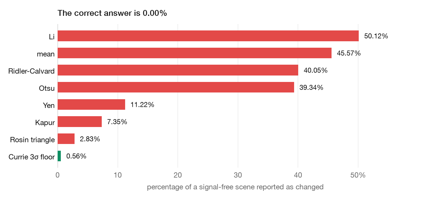
Rosin's triangle performing best of the data-driven selectors is expected, since it is the one designed for a unimodal histogram, and the result corroborates Rosin and Ioannidis, who measured roughly 1% for it. The Currie floor in the last row is not a selector at all, and is the subject of section 6.

4.1 The rate does not decay, it falls off a cliff

The more consequential result is what happens as a real signal appears. I injected a signal occupying 1% of the image and raised its contrast from zero in steps of a quarter of the noise scale, counting false positives only on true-background pixels so that no selector is penalised for finding the thing it was supposed to find.

The step size matters. An earlier version of this experiment sampled contrast at 0, 1, 3, 5, 8, 12 and 20, and the resulting figure showed a smooth diagonal decline. That decline was interpolation between sparse samples, not measurement, and it would have supported the opposite conclusion to the right one.

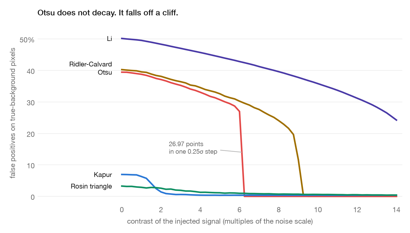
Resolved properly, Otsu does not degrade at all. It holds at 26.98% at a contrast of 6.00 and returns 0.01% at 6.25: a fall of 26.97 percentage points across a single quarter-sigma step. Ridler-Calvard has its own discontinuity later, losing 11.05 points between 9.00 and 9.25. Li has none in this range, its largest single step being 1.16 points, and declines smoothly throughout.

So the honest statement is narrower than "thresholds switch", and more useful: the most widely used selector in the field has two disjoint regimes and no transition between them. Below the cliff it is partitioning noise. Above it, it has locked onto the real signal and the background goes to zero. A pipeline evaluated only on scenes that contain change is evaluated exclusively above the cliff, where it looks perfect, and that measurement carries no information whatsoever about the regime describing most of the earth's surface on most days.

5What a pipeline does on certified ground

Synthetic noise isolates a mechanism. It does not tell you what a real system does to real imagery, where co-registration error, atmosphere, illumination geometry and sensor artefacts all contribute.

I ran a complete change-detection pipeline over the six CEOS-endorsed sites using free Sentinel-2 L2A imagery, at three temporal separations, in two conditions. The calibrated condition is the pipeline as it ships, with an absolute magnitude floor. The no-floor condition sets that floor to zero, leaving the threshold to be chosen purely from the data, which is the condition section 4 characterises. Every pair additionally runs an identity check, comparing a scene against itself, which must return exactly 0.00% or nothing else in the row means anything. Across all 22 successful pairs it did, to four decimal places.

Site geometry comes from the USGS ECCOE catalogue. Each entry gives a centre and two regions of interest; I take a 0.1 degree box centred in the tighter CNES region, because the published 0.2 degree region is about 20 kilometres and would push the analysis grid past its 1024 pixel ceiling, dropping the ground sample to roughly 20 metres. Testing at the sensor's native 10 metres is not optional here, for reasons section 7 makes clear.

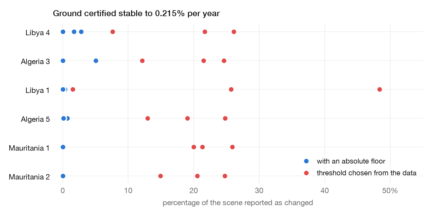
Eighteen pairs across the six certified sites. With the threshold chosen from the data, the median reported change is 21.41%, the mean 20.75%, and the maximum 48.39%, the last being Libya-1 across a 350-day separation. With an absolute floor the same pairs give a median of 0.04%, a mean of 0.62% and a maximum of 5.03%. The separation is roughly five hundredfold at the median, on ground certified stable to 0.215% per year.

Two of the twenty-four attempted pairs were refused outright rather than answered, both at the Lagos harbour control, because no pair in the window cleared the cloud limit over the area of interest. A refusal is a result and is reported as one.

The temporal sweep separates two contributions. Nuisance grows with separation; pipeline error does not. Without the floor, the twenty-day and thirty-five-day pairs already report 25.70% and 7.59%, so most of the error is present immediately and is not a story about the world changing.

6The floor, and where it comes from

The fix for section 4 is not a better selector. It is an absolute one.

This is an old idea with a name worth using, because the name brings a framework. Currie, writing about radiochemistry in 1968, defined the critical level: the signal above which a detection may be declared, derived from repeated measurement of a blank rather than from the sample under test. The construction was later codified in IUPAC recommendations and ISO 11843, and it is the standard vocabulary for detection limits across analytical measurement. Wavelet denoising arrives at the same place from another direction: the universal threshold of Donoho and Johnstone is scaled to the noise level precisely so that, when there is no signal, the estimate is zero.

The change-detection version is max(otsu, min_magnitude), where min_magnitude is an absolute spectral distance rather than a quantile of the present image. In the sweep, a floor three standard deviations above the mean of an independent blank pins the false-positive rate at 0.57% regardless of selector or contrast, while true positives reach 97.7% by a contrast of three standard deviations. It costs almost nothing in sensitivity and removes almost all of the error.

It also makes the choice of selector nearly irrelevant. With the floor applied, Otsu, Li and Rosin's triangle become indistinguishable at low contrast, because in the regime where they disagreed the floor dominates all of them. The floor does not improve the selector. It removes the selector's influence from exactly the region where that influence was harmful.

And it needs the same ingredient the null test needs. A critical level requires an estimate of the noise scale from a signal-free reference; a null test requires a signal-free scene. They are the same acquisition. Once a pipeline has null sites it gets both the measurement and the correction from one place, which is the practical argument for adopting the protocol rather than merely agreeing with it.

7The other half, and a pathology

A detector that reports nothing passes a null test perfectly, so the null test alone is half a measurement. The other half is injection: paint a structure of known ground size into the genuine second acquisition and ask whether the change mask covers it.

Across all six sites and three contrast levels, the detection floor is 50 metres, without exception. That is not a property of the imagery. It is exactly the configured minimum region size of 2,500 square metres, which a 50 metre structure meets precisely. A 40 metre building is 1,600 square metres and is refused before detection is attempted. The sensitivity floor, at these sizes, is a configuration choice rather than a physical limit, and the honest way to report the pair is that the pipeline achieves a median 0.04% false-alarm rate given that it declines to look at anything under 2,500 square metres.

Measuring this correctly required abandoning my first instrument. I began by asking whether injecting a structure raised the total reported change area, and three injections out of 144 said it did the opposite. At Libya-4, a 200 metre structure at high contrast took the reported change from 2.812% to 0.034%. The scene reported thirty times less change once a large real change was added to it.

This is the cliff of section 4.1 appearing in real imagery. The bright structure captures the threshold; the threshold rises onto it; and the pre-existing false positives, which were the entire 2.812%, fall below the new cut and are reclassified as background. Checking the change mask against the injected footprint confirms it: recall over the structure is 1.00 in all three cases. The structure is perfectly detected. The total is nonsense.

The practical consequence deserves stating plainly. For a pipeline in this regime, the reported area of change is not monotonic in the amount of change present, so a user watching that number fall could be watching a large new structure arrive.

8What the protocol found

The case for a validation practice is what it catches. Applied to a working pipeline, the null test surfaced seven defects, listed with an honest assessment of whether anything else would have found them.

Defect	Measured effect	Caught by other means?
Threshold had no absolute floor, so a relative criterion split pure noise	11.21% to 0.67% on the desert control	No. Needs an input whose correct answer is known to be zero
Radiometric normalisation fit over invalid pixels, letting a dominant water surface drag the coefficients	Helped the desert, 20% to 7%; hurt the harbour, 2% to 14.5%	Partly. The sign flip between sites identified the cause
Minimum region size expressed in pixels rather than area	The same setting meant 800 m² at 10 m and 0.7 m² at 30 cm	Yes, in principle, by inspection
Reported ground sample was the sensor's native 10 m while the provider resampled every request to a fixed 256 px tile	A 6 km box was really about 26 m/px; every area figure downstream was wrong	No. Outputs looked reasonable; only an absolute size check exposes it
Catalogue search took a fixed 12 scenes sorted ascending, silently truncating long windows	A one-year request returned a 50-day comparison	No. Needs to expect a specific temporal separation and verify it
Normalisation's degeneracy guard tests scene spread against an absolute 1e-6, so never fires on a uniform target where observed spread is about 1e-3	Gain uncertainty degrades from 0.01% to 1.36% across the uniformity range	No. Appears only on uniform ground
Reported change area is not monotonic in the change present	2.812% to 0.034% when a 200 m structure was added	No. Requires injecting a known structure and watching the total fall

Five of the seven are invisible in the outputs, and four of those require specifically a signal-free or geometrically-known input. The resolution defect is the one that matters most: a ground sample that lies corrupts every square-metre number the system prints, and nothing about the imagery looks wrong.

The normalisation guard is the most interesting, because it is a trap laid by the protocol itself. Radiometric normalisation regresses the second acquisition against the first to recover a gain, and its guard against an unfittable scene compares the spread of the predictor to an absolute constant. On a target selected for spatial uniformity better than 3%, the spread is small but nowhere near that constant, so the guard passes and the gain is estimated from almost no dynamic range. The property that certifies a site as a good null is the property that degenerates the normaliser, which makes this defect not merely findable by null testing but essentially only findable that way.

9What this does not establish

Null sites are bright and arid, and that is a real limitation. Work validating Level-2 surface reflectance against instrumented reference sites has made precisely this objection: the surfaces are much brighter and more uniform than those most downstream applications observe. A false-alarm rate measured over Libya-4 does not transfer to a temperate forest or a cloudy coastline. What it bounds is the pipeline's response to the easy case, and a system that fails the easy case has been usefully convicted, while a system that passes it has proved less than it might appear.

Radiometric stability is not physical stasis. The 0.215% per year figure describes the aggregate top-of-atmosphere signal, not a guarantee that no pixel changed. Sand moves. A null site provides a strong prior that reported change is nuisance rather than event, not a proof, which is why the expectation should be reported rather than assumed to be zero.

The synthetic experiments are idealised. Independent noise, a square target, no co-registration error, no atmosphere. They isolate the mechanism; section 5 is what speaks to the world.

The injection floor is a floor on this configuration. Fifty metres is where the minimum-region setting sits, so the experiment establishes that the configuration binds before the imagery does. It does not establish what the imagery alone could resolve.

And this is one pipeline. The mechanism results in section 4 apply to any system ending in one of those selectors, which is most classical change detection. They say nothing directly about learned detectors, which now dominate the field. Whether a network trained on an annotated benchmark also fails a null test is the obvious next question and it is not answered here. I would expect it to, since nothing in a training objective penalises confident output on an input unlike anything in the training set, but expectation is not measurement, and doing it fairly needs models trained in the same domain rather than a building-detection network pointed at a desert.

10Reproducing this

The mechanism sweep is numpy and scikit-image and runs in under a minute on a laptop. The field measurement needs no API key, no registration and no GPU: Sentinel-2 L2A is free and the site coordinates are public. Fixed seeds throughout, with the environment recorded in the result files.

The artifact that matters is not this note. It is the protocol, the site list and the harness, released so that somebody else can run their own detector against the same ground and publish their own number. A paper arguing for a benchmark is a poor substitute for a benchmark anyone can run.

References

Verified against fetched source text. Where a full text was unreachable, metadata was confirmed through Crossref and the limitation noted.

1. N. Otsu. A threshold selection method from gray-level histograms. IEEE Transactions on Systems, Man, and Cybernetics, SMC-9(1):62–66, 1979.
2. P. L. Rosin. Unimodal thresholding. Pattern Recognition, 34(11):2083–2096, 2001.
3. P. L. Rosin and E. Ioannidis. Evaluation of global image thresholding for change detection. Pattern Recognition Letters, 24(14):2345–2356, 2003.
4. J. Zack, W. E. Rogers and S. A. Latt. Automatic measurement of sister chromatid exchange frequency. Journal of Histochemistry and Cytochemistry, 25(7):741–753, 1977.
5. M. Sezgin and B. Sankur. Survey over image thresholding techniques and quantitative performance evaluation. Journal of Electronic Imaging, 13(1):146–165, 2004.
6. X. Xu, S. Xu, L. Jin and E. Song. Characteristic analysis of Otsu threshold and its applications. Pattern Recognition Letters, 32(7):956–961, 2011.
7. Z. Hou, Q. Hu and W. L. Nowinski. On minimum variance thresholding. Pattern Recognition Letters, 27(14):1732–1743, 2006.
8. L. A. Currie. Limits for qualitative detection and quantitative determination. Analytical Chemistry, 40(3):586–593, 1968.
9. D. L. Donoho and I. M. Johnstone. Ideal spatial adaptation by wavelet shrinkage. Biometrika, 81(3):425–455, 1994.
10. A. Desolneux, L. Moisan and J.-M. Morel. Edge detection by Helmholtz principle. Journal of Mathematical Imaging and Vision, 14:271–284, 2001.
11. J. R. Schott, C. Salvaggio and W. J. Volchok. Radiometric scene normalization using pseudoinvariant features. Remote Sensing of Environment, 26(1):1–16, 1988.
12. H. Cosnefroy, M. Leroy and X. Briottet. Selection and characterization of Saharan and Arabian desert sites for the calibration of optical satellite sensors. Remote Sensing of Environment, 58(1):101–114, 1996.
13. N. Khadka, C. Teixeira Pinto and L. Leigh. Detection of change points in pseudo-invariant calibration sites time series using multi-sensor satellite imagery. Remote Sensing, 13(11):2079, 2021.
14. F. D. Tuli, C. Teixeira Pinto, X. Jing, L. Leigh and D. Helder. New approach for temporal stability evaluation of pseudo-invariant calibration sites. Remote Sensing, 11(12):1502, 2019.
15. D. L. Helder, K. J. Thome, N. Mishra, G. Chander, X. Xiong, A. Angal and T. Choi. Absolute radiometric calibration of Landsat using a pseudo invariant calibration site. IEEE Transactions on Geoscience and Remote Sensing, 51(3):1360–1369, 2013.
16. C. Bacour, X. Briottet, F.-M. Bréon, F. Viallefont-Robinet and M. Bouvet. Revisiting pseudo invariant calibration sites over sand deserts. Remote Sensing, 11(10):1166, 2019.
17. P. Olofsson, G. M. Foody, M. Herold, S. V. Stehman, C. E. Woodcock and M. A. Wulder. Good practices for estimating area and assessing accuracy of land change. Remote Sensing of Environment, 148:42–57, 2014.
18. N. Gonthier. Operational change detection for geographical information: overview and challenges. arXiv:2503.14109, 2025.
19. Y. Chen, O. Y. Gnedin, A. Price-Whelan et al. StarStream: automatic detection algorithm for stellar streams. arXiv:2510.14929, 2025.
20. Planck Collaboration. Planck 2015 results III: LFI systematic uncertainties. arXiv:1507.08853, 2015.
21. B. Pflug, J. Louis, R. de los Reyes et al. Evaluation of Sen2Cor surface reflectance products over land surface with reference measurements on ground. IGARSS 2022, 4308–4311.
22. B. A. Franz, S. W. Bailey, P. J. Werdell and C. R. McClain. Sensor-independent approach to the vicarious calibration of satellite ocean color radiometry. Applied Optics, 46(22):5068–5082, 2007.
23. CEOS WGCV LPV. Land cover and change map accuracy assessment and area estimation good practices protocol, v1.1, 2025.
24. USGS EROS CalVal Center of Excellence. Test sites catalogue, calval.cr.usgs.gov, accessed 22 September 2026.